Supervised ML: Classification Algorithms

Supervised Machine Learning Algorithms

Scikit-learn: Classification Algorithms.

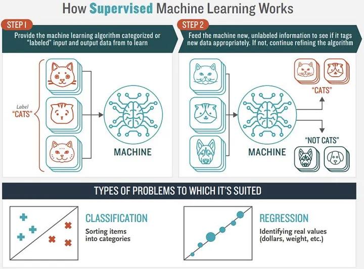
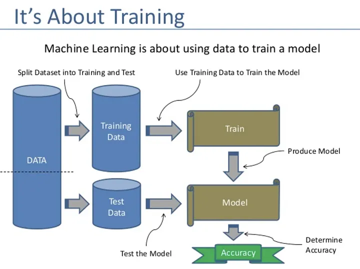
Scikit-learn is a very popular open-source machine learning library based on Python. It supports a variety of supervised (regression and classification) and unsupervised learning models.

Image credits: Jorge Leonel. Medium

One list of 10 classification algorithms from Scikit-Learn, that we need to consider.

1. Logistics Regression

from sklearn.linear_model import LogisticRegression

2. Support Vector Machine

from sklearn.svm import SVC

3. Naives Bayes (Gaussian Multinomial)

from sklearn.naive_bayes import GaussianNB
from sklearn.naive_bayes import MultinomialNB

4. Stochastic Gradient Descent Classifier

from sklearn.linear_model import SGDClassifier

5. KNN (k-nearest neighbor)

from sklearn.neighbors import KNeighborsClassifier

6. Decision Tree Learning

from sklearn.tree import DecisionTreeClassifier

7. Random Decision Forest

from sklearn.ensemble import RandomForestClassifier

8. Gradient Boosting Classifier

from sklearn.ensemble import GradientBoostingClassifier

9. LightGBM Classifier

from lightgbm import LGBMClassifier

10. XGBoost Classifier

from xgboost.sklearn import XGBClassifier

Classification. Classification is an algorithm for predicting to which set of items, classes or categories an object belongs to. Some examples of Classification algorithms:

• Logistic Regression
  
• Support Vector Machines
  
• Naive Bayes
  
• Stochastic Gradient Descent
  
• K-Nearest Neighbors Classifier
  
• Decision Tree Classifier
  
• Random Decision Forest Classifier
• Gradient Boosting Classifier
• LightGBM Classifier (Microsoft)
• XGBoost Classifier

---

Supervised Learning Evaluation

Classifier evaluation metrics:

• Precision and Recall.
• Precision = TP/(TP + FP), is the ratio of the correctly identified positive cases to all the predicted positive cases.
• Recall = TP/(TP + FN), also known as sensitivity, is the ratio of the correctly identified positive cases to all the actual positive cases.
• Accuracy. Accuracy is a statistical measure that is defined as the quotient of correct predictions (both True positives (TP) and True negatives (TN)) made by a classifier divided by the sum of all predictions made by the classifier, including False positives (FP) and False negatives (FN). Accuracy = (TP + TN)/(TP + TN + FP + FN).
• F1-score. F1 = 2(Precision * Recall)/(Precision + Recall) = 2TP/(2TP + FP + FN).
• Area under the curve - AUC
• The Confusion Matrix, is a specific table layout that allows visualization of the performance of an algorithm

Sklearn.metrics

The scikit-learn library includes a large collection of classification metrics that can be used for measuring the performance of the algorithms.

• sklearn.metrics.PrecisionRecallDisplay
• sklearn.metrics.precision_score
• sklearn.metrics.recall_score
• sklearn.metrics.accuracy_score
• sklearn.metrics.f1_score
• sklearn.metrics.roc_auc_score
• sklearn.metrics.ConfusionMatrixDisplay

---

Jupyter Notebook Example

Please open this Notebook in Google Colab.

---

Classification Algorithms using R.

Example R code for creating and comparing K-nearest neighbors, Decision Tree, and Support Vector Machine classification models, including splitting into training and testing data, scaling numerical variables, confusion matrix, and ROC curve:

# Load required packages
library(caret)
library(pROC)
library(e1071)
library(rpart)

# Load data and split into training and testing sets
data <- read.csv("dataset.csv")
set.seed(123)
trainIndex <- createDataPartition(data$target, p=0.8, list=FALSE)
trainData <- data[trainIndex, ]
testData <- data[-trainIndex, ]

# Scale numerical variables in the training and testing sets
preProcValues <- preProcess(trainData[,c("num_var1", "num_var2")], method=c("center", "scale"))
trainData[,c("num_var1", "num_var2")] <- predict(preProcValues, trainData[,c("num_var1", "num_var2")])
testData[,c("num_var1", "num_var2")] <- predict(preProcValues, testData[,c("num_var1", "num_var2")])

# Train the K-nearest neighbors model with k=5
knnModel <- train(target ~ num_var1 + num_var2 + cat_var1 + cat_var2, data=trainData, method="knn", preProcess=c("center", "scale"), tuneLength=10, trControl=trainControl(method="cv", number=10), metric="Accuracy", tuneGrid=data.frame(k=seq(1,20,2)))

# Train the Decision Tree model
dtModel <- train(target ~ num_var1 + num_var2 + cat_var1 + cat_var2, data=trainData, method="rpart", preProcess=c("center", "scale"), tuneLength=10, trControl=trainControl(method="cv", number=10), metric="Accuracy")

# Train the Support Vector Machine model
svmModel <- svm(target ~ num_var1 + num_var2 + cat_var1 + cat_var2, data=trainData, kernel="linear", cost=1)

# Make predictions on the testing set for all models
knnPredictions <- predict(knnModel, testData)
dtPredictions <- predict(dtModel, testData)
svmPredictions <- predict(svmModel, testData)

# Calculate confusion matrix for all models
knnConfMatrix <- confusionMatrix(knnPredictions, testData$target)
dtConfMatrix <- confusionMatrix(dtPredictions, testData$target)
svmConfMatrix <- confusionMatrix(svmPredictions, testData$target)

# Print confusion matrix for all models
print("K-Nearest Neighbors Confusion Matrix")
print(knnConfMatrix$table)
print("Decision Tree Confusion Matrix")
print(dtConfMatrix$table)
print("Support Vector Machine Confusion Matrix")
print(svmConfMatrix$table)

# Plot ROC curve for all models
knnROC <- roc(testData$target, predict(knnModel, testData, type="prob")[,2])
dtROC <- roc(testData$target, predict(dtModel, testData, type="prob")[,2])
svmROC <- roc(testData$target, predict(svmModel, testData, type="decision"), levels=c("0", "1"))

par(mfrow=c(1,3))
plot(knnROC, main="K-Nearest Neighbors ROC Curve", print.auc=TRUE)
plot(dtROC, main="Decision Tree ROC Curve", print.auc=TRUE)
plot(svmROC, main="Support Vector Machine ROC Curve", print.auc=TRUE)

Classification metrics in R example

# Load required packages
library(caret)

# Load data and split into training and testing sets
data <- read.csv("dataset.csv")
set.seed(123)
trainIndex <- createDataPartition(data$target, p=0.8, list=FALSE)
trainData <- data[trainIndex, ]
testData <- data[-trainIndex, ]

# Train the classification model (e.g. K-nearest neighbors)
model <- train(target ~ num_var1 + num_var2 + cat_var1 + cat_var2, data=trainData, method="knn", preProcess=c("center", "scale"), tuneLength=10, trControl=trainControl(method="cv", number=10), metric="Accuracy", tuneGrid=data.frame(k=seq(1,20,2)))

# Make predictions on the testing set
predictions <- predict(model, testData)

# Compute confusion matrix
confMatrix <- confusionMatrix(predictions, testData$target)
print("Confusion Matrix")
print(confMatrix$table)

# Compute accuracy
accuracy <- confMatrix$overall["Accuracy"]
print(paste("Accuracy:", accuracy))

# Compute sensitivity/recall
sensitivity <- confMatrix$byClass["Sensitivity"]
print(paste("Sensitivity/Recall:", sensitivity))

# Compute specificity
specificity <- confMatrix$byClass["Specificity"]
print(paste("Specificity:", specificity))

# Compute precision
precision <- confMatrix$byClass["Precision"]
print(paste("Precision:", precision))

# Compute F1 score
f1Score <- confMatrix$byClass["F1"]
print(paste("F1 Score:", f1Score))

---

References

• Scikit-learn cheat sheet: methods for classification & regression. Aman Anand.
• 10 Classification Methods from Scikit-learn we should know. Prosenjit Chakraborty.
• Top 6 Machine Learning Algorithms for Classification. Destin Gong. Towards Data Science, Medium.
• How to explain the ROC curve and ROC AUC score?

---

Created: 02/09/2023 (C. Lizárraga); Last update: 01/19/2023 (C. Lizárraga)

CC BY-NC-SA