Just copy the scripts. You must have python and R installed.
This repository contains R scripts for visualizing word spaces based on the analysis of word frequency distributions. The visualization is designed to reveal semantic similarity within the distribution of words, especially named entities, or "hero words", assuming a Negative Binomial Distribution of them. For each word, a pair of parameters is calculated, namely NBD parameters k and p, and they can be viewed as word embeddings induced from a text corprus.
Visualize word embeddings in 2D or 3D space so that you can examine the spatial relationships between words and inspect clusters or semantic groupings. The resulting plots provide insights into the relation of words inside the corpus, aiding in the exploration of key themes and relationships among words. Set filters to view main heros or remarkable background content words. This can be useful when one needs to visualize keywords, or feature words, even within a small collection of homogenious texts, such a novel.
Of course, you can use the NBD technique also for larger collections of texts, such as medical articles, e-mails, user reviews, news. There really no limit of how large a collection of texts can be, but it is essencial that the corpus itself is meaningful.
gutenberg.py Download and parse any Project Gutenberg book to prepare for analysis with wordstats.py
compress.py: Combines txt files into a "corpus", performs elementary parsing, and removes punctuation marks. The processed text is then saved for further analysis.
wordstats.py: Prepares word frequency lists. The results are saved to a text file.
ngramstats.py: Prepares bigram frequency lists. The results are saved to a text file.
calculate.py: Get some corpus linguistics statistics from word frequencies using Python only (no R)
fit.R: R script to estimate k and p parameters for NBD (Negative Binomial Distribution) assuming that word frequency distributions follow NBD
plot.R: R script to draw plots from data prepared by fit.R
plot3D.R: R script to draw 3D plots from data prepared by fit.R
plot3D2.R: Plot3D2.R offers improved visualisation of input data. It creates 3D scatterplot and allows for control of data filters.
Get a book to analyze. Edit the script with the required URL from Project Gutenberg. A book is treated as a 'corpus', so each book chapter is viewed as a text in a collection of texts.
If you already have your texts that you want to analyze, combine them and prepare corpus.txt, the corpus file:
bash
python ~/corpus_utils/compress.py /path/to/texts corpus.txt
This script takes text files from the specified directory, combines and parses them.
Count word frequencies:
bash
python ~/corpus_utils/wordstats.py corpus.txt frequencies.txt 3 10000
Here, min word token frequency is 3, max word token frequency is 10000. For larger corpora it is recommended to set min frequency to a larger value.
Notice, you should not skip this step if you want to run NBD fitting with R scripts below.
Count bigram frequencies:
bash
python ~/corpus_utils/bigramstats.py corpus.txt frequencies.txt 10 10000
Here, min bigram frequency is 10, max word token frequency is 10000. For larger corpora it is recommended to set min frequency to a larger value.
Notice, you should not skip this step if you want to run NBD fitting with R scripts below.
Now data is prepared by wordstats.py and we can calculate sum, mean, variance, and dispersion for each word-token. Input file, frequencies.txt, must be space-separated. Use this script only if you do not have R, otherwise skip this step.
bash
python ~/corpus_utils/calculate.py frequencies.txt final_stats.txt
This script calculates sum (TF), mean, variance, and dispersion for each word and it also estimates Negative Binomial Parameters k and p using method of moments. These estimations are infrerior to Maximum likelihood (MLE) method, but they are easy to implement in Python. Input is read from space-separated file (word matrix) prepared by wordstats.py. Document frequency (DF), TF*IDF, and entropy are also calculated using this script.
Using data prepared by wordstats.py we can estimate k and p parameters for NBD. Calculate sum for each word-token (absolute Word Frequency) and Document Frequency (DF). This is a compute-intensive operation and may take some time, especially for a larger dataset. Run at your own risk.
bash
Rscript ~/corpus_utils/fit.R frequencies.txt results.tab
Please, run fit2.R to prepare data for 3D plot below. For 2D plot, run fit.R.
Plot.R creates scatterplot from data, which was prepared using fit.R
bash
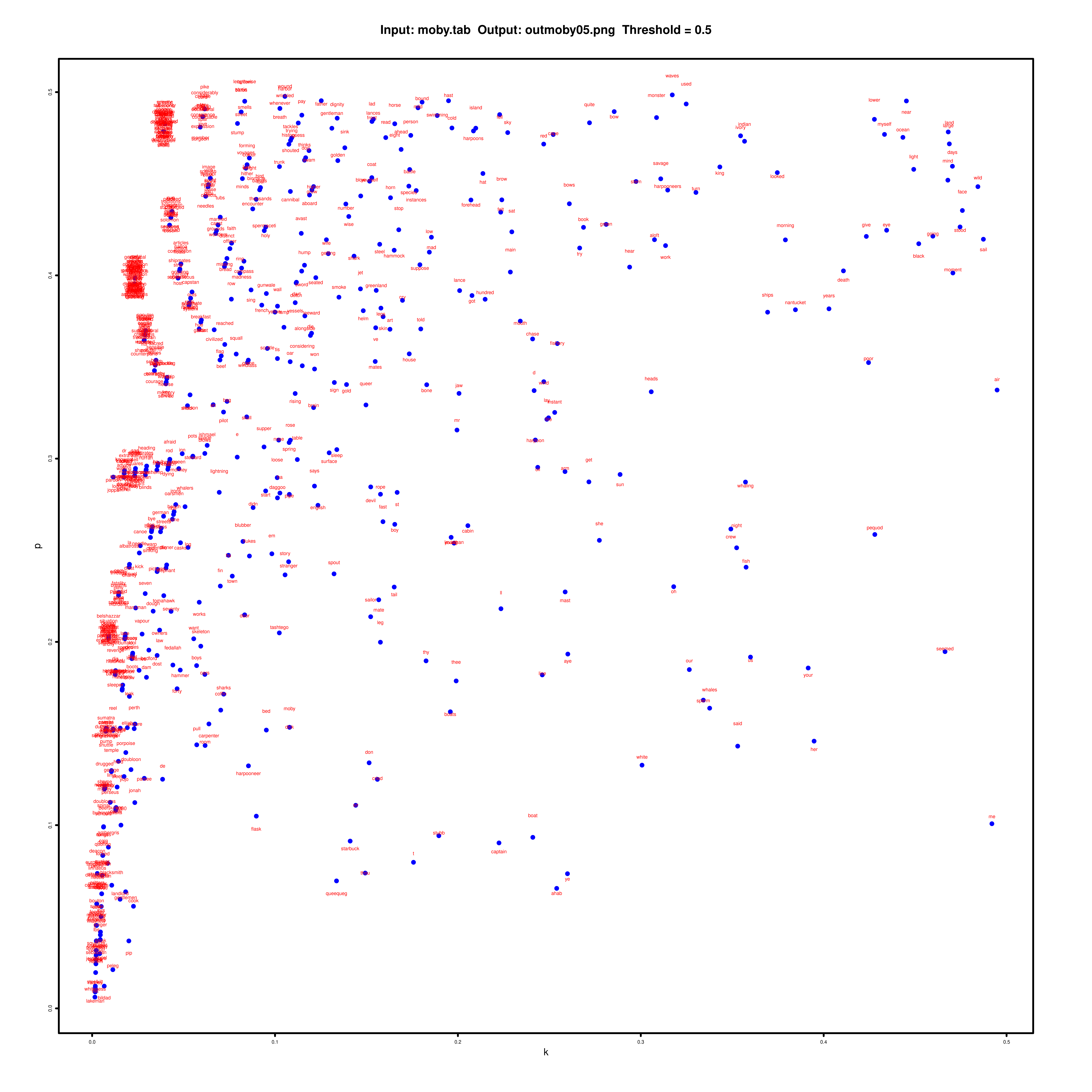
Rscript plot.R input.txt output.png 0.5
In this example, 0.5 is thresholp value of NBD parameters k and p. Try experimenting with this value to zoom in and out of the plot. Interesting values are between 0.1 and 0.7, see graphs in the repo.
This plot shows 2D visualisation of Melville's Moby Dick with such settings:
Plot3D.R creates 3D scatterplot from data, which was prepared using fit.R, where x axis is parameter k, y - parameter p, and z - Document Frequency (DF) The higher the DF, the more texts in the coprus contain the word. So, widespread words have higher DF value. This is not to be confused with absolute frequency of the word, measured by 'sum' in data prepared with fit.R
bash
Rscript plot3D.R input.txt output.png 20 0.1
In this example, 20 is rotation angle of the scatterplot, 0.1 is thresholp value of NBD parameters k and p. Try experimenting with this value to zoom in and out of the plot. Interesting values are between 0.1 and 0.7, see graphs in the repo.
First, prepare data with fit2.R. fit2.R is similar to fit2.R, but offers more functionality (calculated DF and other values).
bash
Rscript plot3D2.R input.txt output.png 300
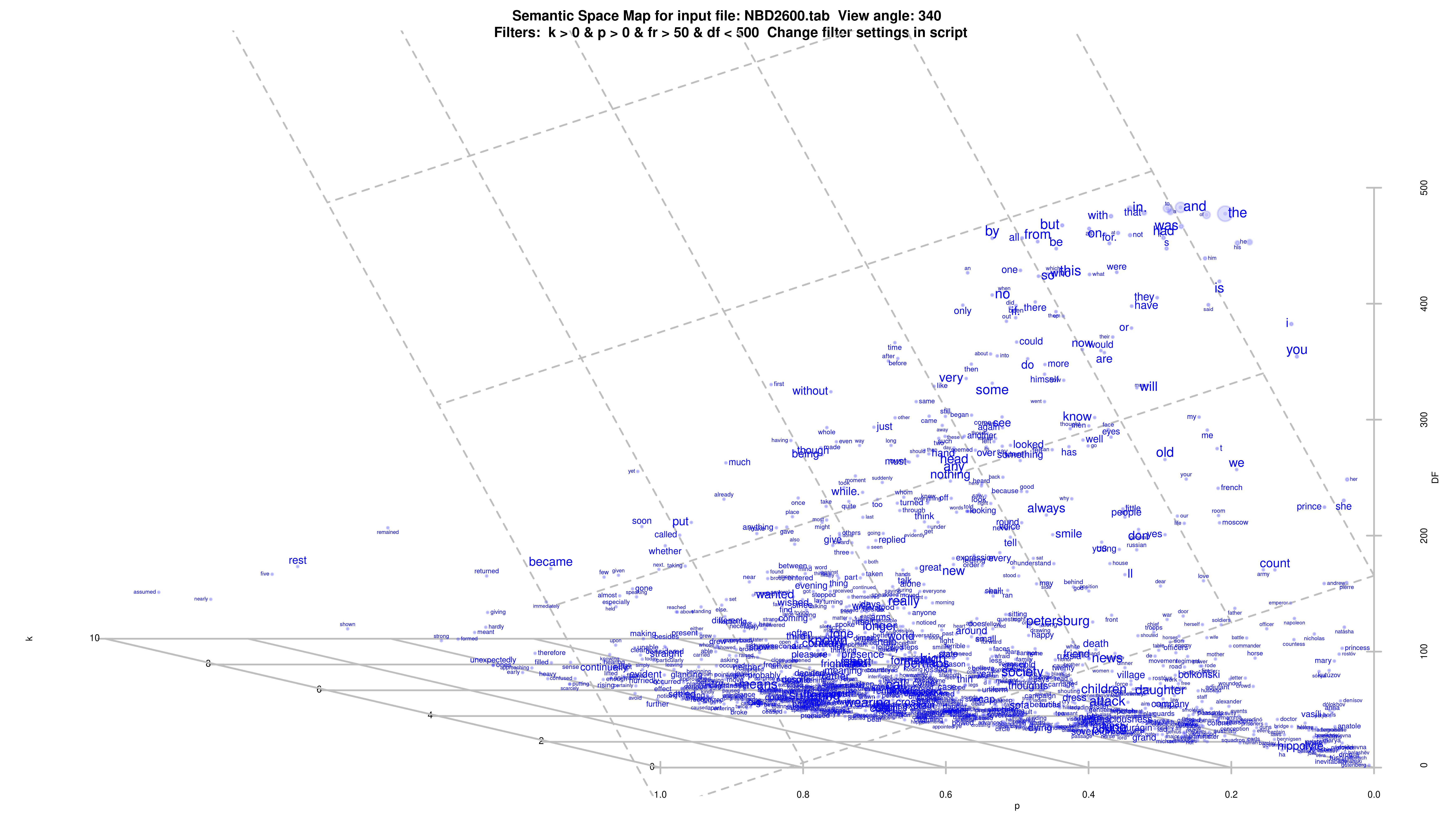
Here, 300 is the projection angle. Try experimenting with this value to look around. Z-axis id Document Frequency (DF), the higher the value, the more individual texts in the corpus (your collection) contain the word. X and Y are NBD parameters induced from data generated by plot.R
Inside the script you can set filters. It comes handy to zoom in and out of your data or show a particular segment on the plot.
Filter vars explanation:
- fr is Word Frequency
- df is Document Frequency
- k and p are NBD parameters
Some examples how you can set filters:
- Values to map all data: k > 0 & p > 0 & fr > 1 & df > 1
- Values to map content background words: k > 5 & p > 0.8
- Values to map names of heros: k < 0.1 & p < 0.1
Say, you have a collection of 500 texts. You only want to see data for tokens that meet conditions:
k > 0 & p > 0 & fr > 50 & df < 250 # Word frequency is over 50, and the word is met in half of texts.
Example with k > 0 & p > 0 & fr > 50 & df < 500 for Tolstoy's "War and Peace", image is zoomable.
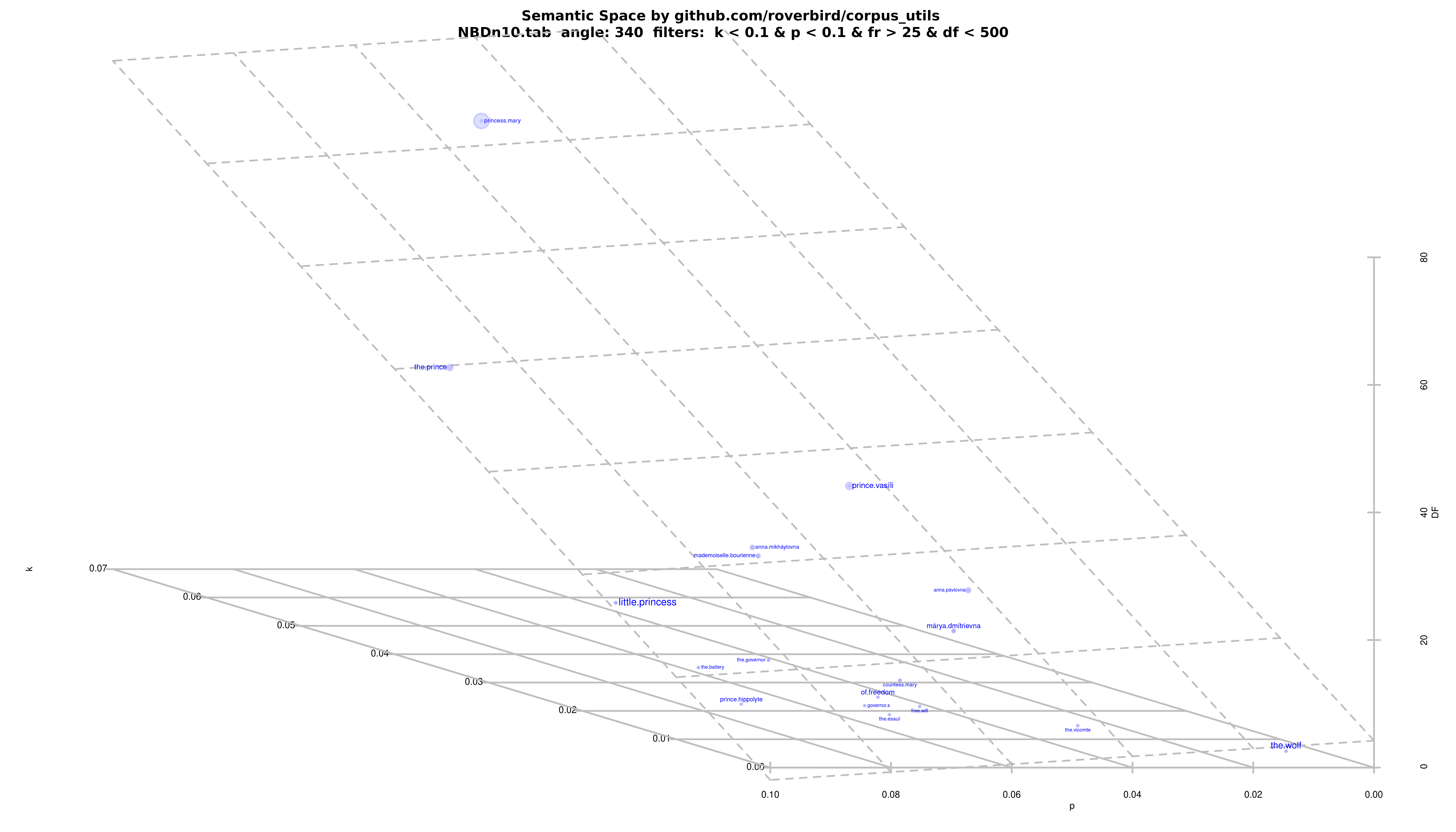
Example with "War and Peace", filter settings to "hero": : k < 0.1 & p < 0.1 & fr > 25 & df < 500.
Example with "War and Peace" n-grams (bi-grams, 2-grams) and filter settings to "hero": k < 0.1 & p < 0.1 & fr > 25 & df < 500. Plot created with plot3D2.R and data prepared with ngramstats.py and fit2.R.
There are directories with addons. texts: this is how individual text can look before you combine them in to a corpus file with compress.py examples/corpora: a readily prepared corpus of fairy tales, you can run wordstats.py, fit.R and plot.R on it examples/graphs: graphs from fairy tales corpora generated by plot.R
Semascope 👁️ is a JavaScript-based text visualization tool that utilizes Plotly JS to graphically represent relationships between words in a collection of texts. The tool, available at plotly_semascope provides an interactive 3D scatter plot where each point represents a word, and the axes correspond to statistical properties of the words extracted with corpus_utils.
Explore the corpus_utils and plotly_semascope in action at textvisualization.app.
The scripts in this repository reproduce the following research:
Title: The Negative Binomial Model of Word Usage Authors: Nina Alexeyeva, Alexandre Sotov Abstract: How people make texts is a rarely asked but central question in linguistics. From the language engineering perspective texts are outcomes of stochastic processes. A cognitive approach in linguistics holds that the speaker’s intention is the key to text formation. We propose a biologically inspired statistical formulation of word usage that brings together these views. We have observed that in several multilingual text collections word frequency distributions in a majority of non-rare words fit the negative binomial distribution (NBD). However, word counts in artificially randomized (permuted) texts agree with the geometric distribution. We conclude that the parameters of NBD deal with linguistic features of words. Specifically, named entities tend to have similar parameter values. We suggest that the NDB in natural texts accounts for intentionality of the speaker.
DOI Code: 10.1285/i20705948v6n1p84
Keywords: word frequency; negative binomial distribution (NBD); text randomization


