-
Notifications
You must be signed in to change notification settings - Fork 26
tech_image states
First we'll lay some ground work for digital imaging, going from scene to display with a few stops in between.
Digital Image
A generic term for a two dimensional grid of picture elements known as "pixels", each containing a numeric representation of intensity. A digital image is commonly composed of 3 individual channels representing red green and blue colored light intensity.Digital images can store a wide variety of data. Different data types like integer and float, different encodings of intensity like log or linear, different representations of color like RGB or HSV.
I will use the term "image" throughout to refer generically to a two dimemsional grid of pixels storing intensity data.
We should however make a distinction between an image that is merely storing pixel intensity data, and an image which has been "rendered" for presentation on a display device. I will try to refer to the first as "image data" and the second as "rendered image".
An image begins its life as a glimmer in the eye of a camera. Photons are projected through a lens and gathered in photosites on a digital sensor.
Each photosite has a color filter which captures a weighted range of the spectrum. There are 3 types of photosites corresponding to the wavelengths which we perceive as red, green, and blue light. Photons from these wavelengths are counted by the photosites and converted into a digital signal representing light intensity.
This sensor is sometimes called a CFA or Color Filter Array. The photosites on the sensor are usually arranged in a specific pattern called a Bayer filter mosaic.
There are more green photosites than red and blue. To turn this bayer mosaic into a image data, we must interpolate red green and blue pixel values from the bayer array. There are many specialized debayer algorithms designed to squeeze the best possible resolution out of the bayer data, while avoiding artifacts.
If we plot the response of each color filter over the spectrum of visible light, we can see the spectral response of the camera sensor. Here is the spectral response of the Canon 5D mk3, captured by Scott Dyer from ACES.
We could think of this as representing the spectral response of the Camera Observer.
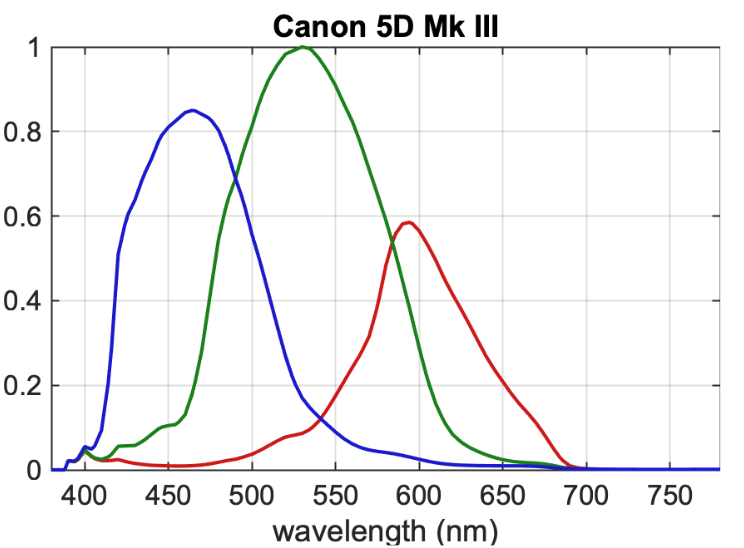
The spectral response of a camera is similar to the human eye. There are three photosites sensitive to specific ranges of the electromagnetic spectrum. However the response of the photosites is not exactly the same as the cones in our eye.
The Human Observer has a different spectral response than a camera.
Since the spectral response of the camera observer is different from that of a human observer, the color will not look "correct" to our eyes directly off of the CFA. We must apply some transformations to the color from the camera sensor so that it looks "correct" to our human eyeballs.
The most commonly used process is to calculate a 3x3 matrix using a linear regression analysis fit. This 3x3 matrix takes camera color and distorts it to find the best fit for a set of commonly occurring reflected scene colors, like those in a macbeth chart. After the 3x3 matrix is applied, the result will be a reasonably good fit for colors near the macbeth chart sample points, but will have more and more error the further out you go.
This 3x3 matrix is what is called an IDT or "Input Device Transform" in the ACES system. For digital still cameras, this IDT matrix is usually included in the raw file. When you debayer, it is automatically applied to get correct looking color in the resulting image.
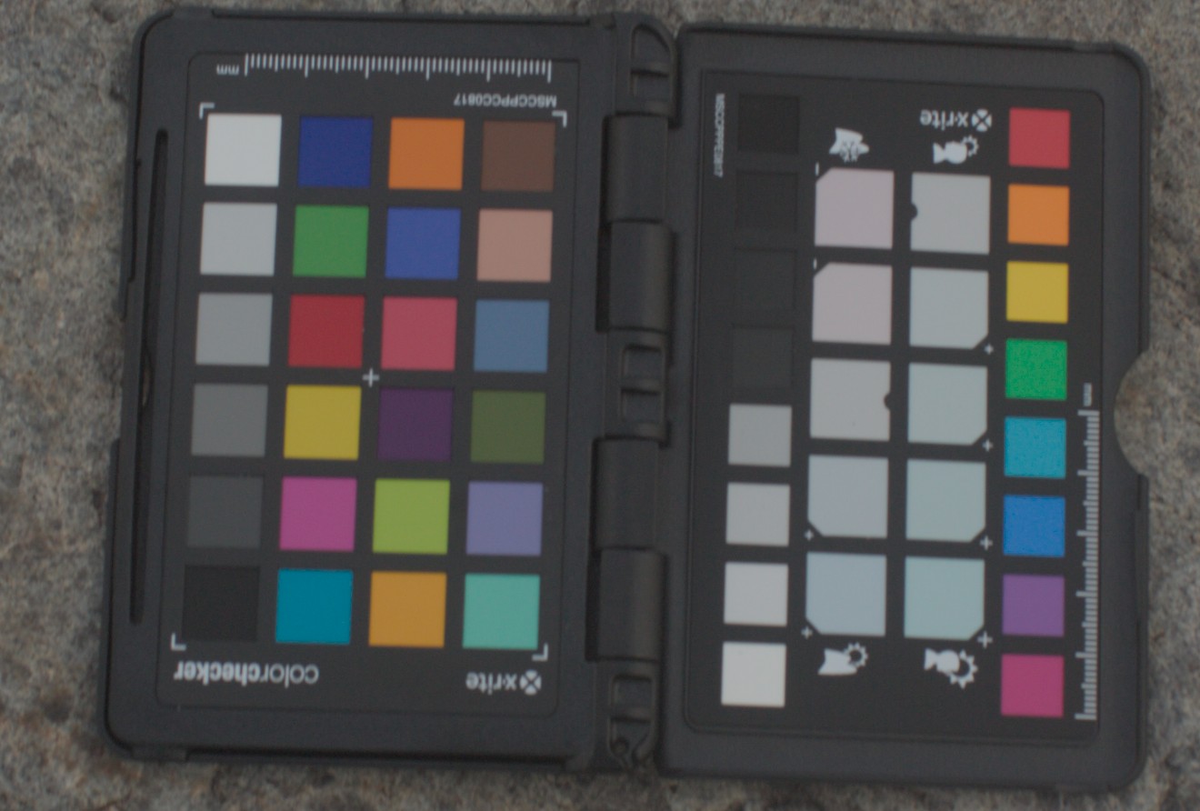
Here is an example photograph of a macbeth chart taken with a 5D mk3 digital still camera.
Debayered with the dcraw_emu software included with LibRaw, and displayed with OpenDRT.
dcraw_emu -4 -T -q 4 -dcbe -o 6 <file.cr2>
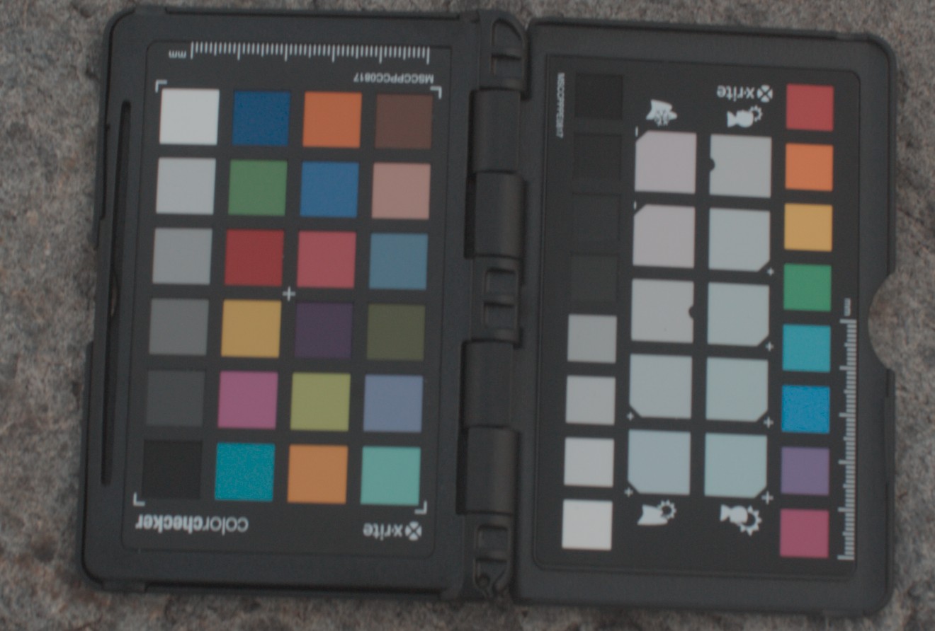
Here is the same image, but debayered without the IDT applied. See how the colors look wrong?
dcraw_emu -4 -T -q 4 -dcbe -o 0 <file.cr2>
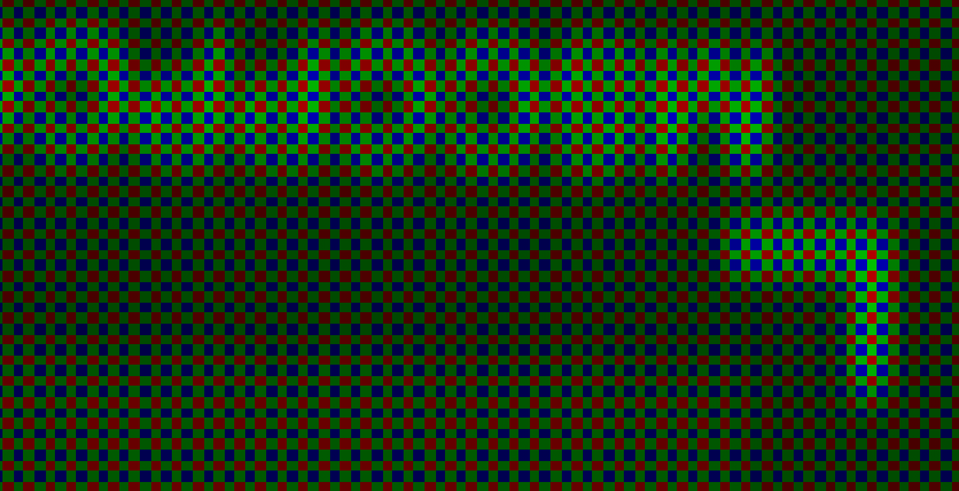
And here is the same image without the debayer step. This shows the bayer mosaic pattern. The raw data captured by the photosites on the sensor.
dcraw_emu -4 -T -disinterp -o 0 <file.cr2>
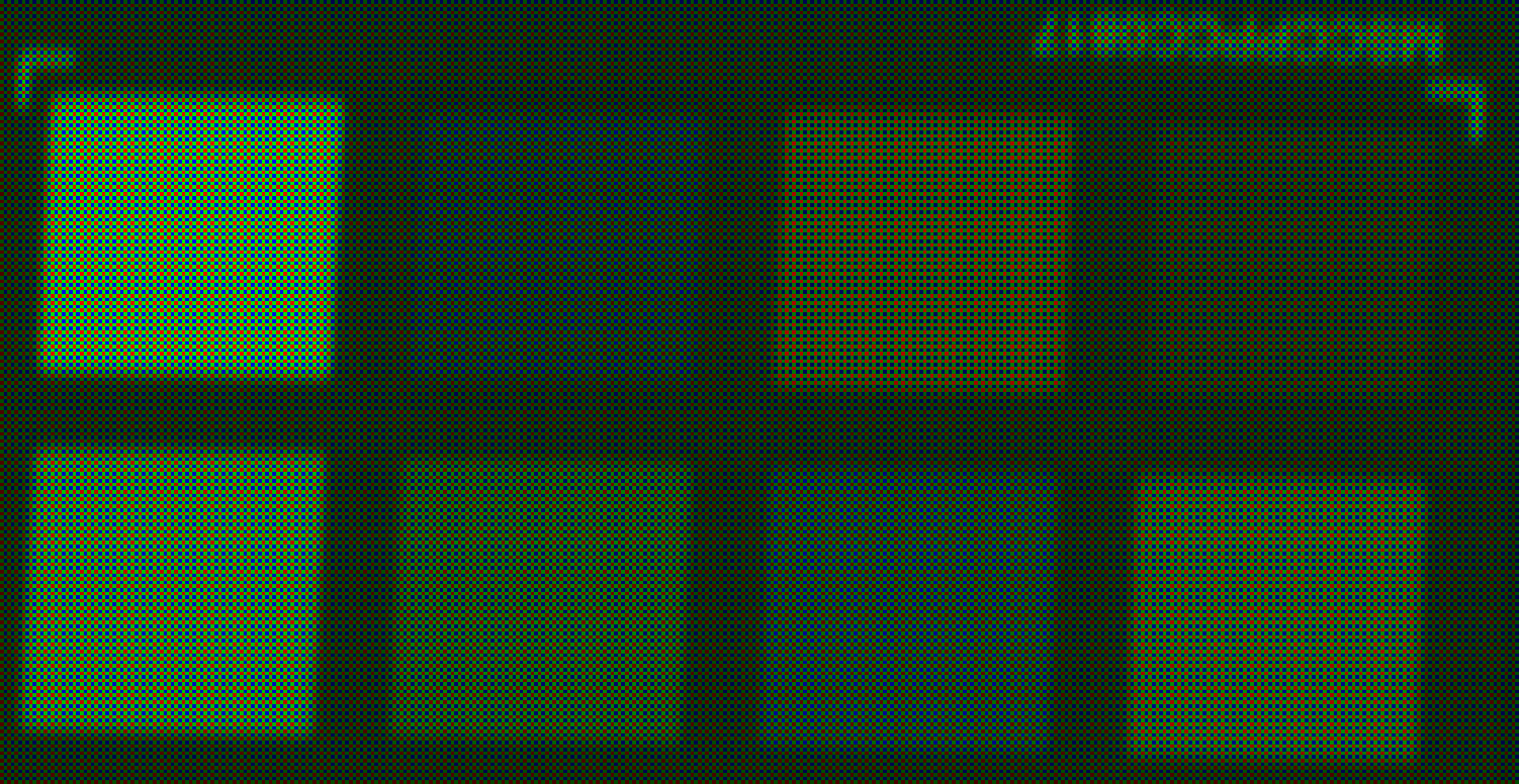
And a detail view
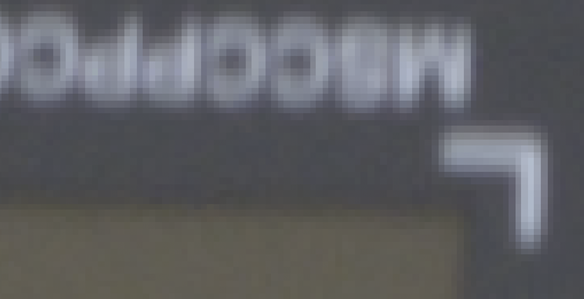
And the final interpolated pixels.
We have talked about how color information is handled in the conversion from bayer mosaic data into pixel data. Now we will put aside concerns of color, and talk a bit more specifically about a sensor's response to light intensity.
Digital camera sensors have a linear response to light. As you increase the number of photons, the value of the recorded pixel increases by the same amount. 2x the light means 2x the signal.
An image can be called Scene-Referred if there is a known mathematical relationship between the captured pixel data, and the original intensity of light in the scene.
More specifically, an image can be called Scene-Linear if there is a proportional relationship between pixel value and scene light intensity. So if we are working with a scene-linear image, we can expose that image up or down, and the image is still scene-linear. However, if we apply a power function or a curve to that image, scene-linearity will be broken.
Camera log encodings can also be called scene-referred. Say we have a 10-bit DPX storing integer code values between 0 and 1023. This image contains an Alexa V3 LogC transfer function of the original scene-linear image values. This image is still scene-referred because we can easily get back to the scene-linear values, without losing much quality.
Scene-linear is very important for many domains of image processing. For correct motionblur, defocus, convolution, and for integrating rendered cg images, it is very important to have pixel values which represent the light intensity of the scene.
So if we are doing any kind of serious work on our images, we want to preserve scene-linearity. When we decode the raw image from the camera, it is very easy to preserve linearity, because the sensor data itself is linear. It is usually a two-step process.
- Decode the bayer mosaic data into image data.
- Set exposure so that an 18% diffuse reflector is positioned at a scene-linear value of about 0.18. This value is sometimes referred to as middle grey.
(Note: it's not really this simple. Exposure is a creative choice. See this excellent discussion of exposure by Mark Vargo). - Store this data in an image format which can support scene-linear floating point data, like a 16 bit half float OpenEXR.
The real world has a very large range of light intensity. From radiation on the surface of the sun that would melt your face off, to absolute zero molecular motion in the void of inter-galactic space and everything in between.
Camera sensors have a more limited range. There is a lower threshold below which the sensor just captures noise, and an upper threshold above which the sensor can not record any more detail. The range from noise floor to sensor clip is called the dynamic range. Because the range of light intensity is so large, it's useful to have a logarithmic scale. We use stops. A stop is one doubling of light. The dynamic range of a camera is usually expressed as the number of stops above and below middle grey.
With scene-linear data we have a reasonable representation of light intensity as seen by the camera observer. But as image makers we are sitting at a desk in front of a display device. That display device is not capable of producing the same luminance as real lights in a scene. If we want to display the entire range of image data captured by the camera, we must compress and reduce it. This "rendering" is what this project is all about.
An image can be called Display-Referred if it has a known mathematical mapping between between pixel value and light emitted from a display device.
This "display rendering" is highly nonlinear and involves many complex processes and choices, both creative and technical. Doing work on an image after display rendering is problematic.
The process of display rendering can also be thought of as "lossy". Once a display rendering is applied, it is impossible to get back to the original scene data without loss of quality. It is healthy to think of a display rendering as a one-directional forward transform. Inverse display transforms are possible, but they are problematic and to be avoided if possible.
We can think of the display transform as the window we look through to see our captured image data. Since working with the scene-linear image data has the most advantages, it makes sense to defer the display transform to be as late as possible in the image processing chain. This allows us to preserve the most information for as long as possible.
Scene-linear colorspaces can be thought of as unbounded: they have no theoretical upper or lower limit. Display-referred colorspaces on the other hand, are bounded. Pixel values exist in limited range between 0 and 1. But maybe this is all a bit abstract. Let's see if there's a better way to visualize what this means.
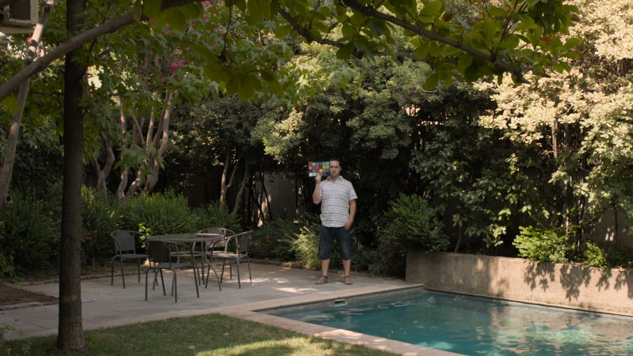
Let's take this test image of a guy next to a pool, from cinematographery.net (here rendered through OpenDRT).
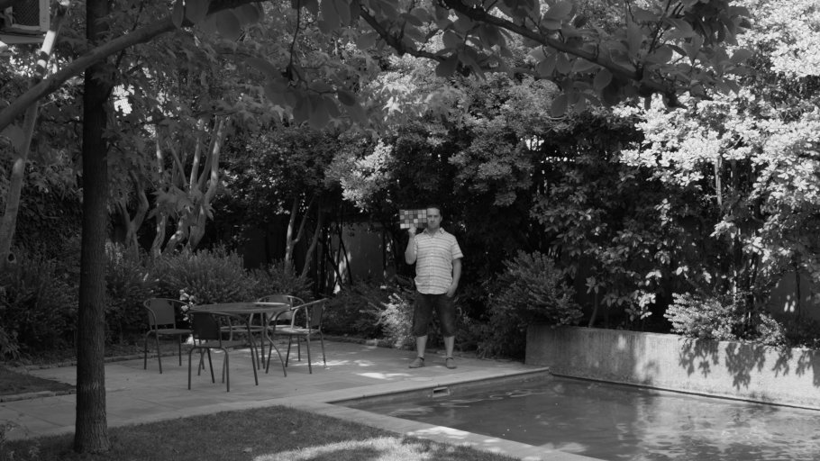
We could visualize the intensity of the scene-linear pixels by taking the luminance of the pixels: L = r*0.268064+g*0.672465+b*0.0594715 (Rendered through OpenDRT for display again)
If we plot this in 3 dimensions using luminance as height, it might look something like this:
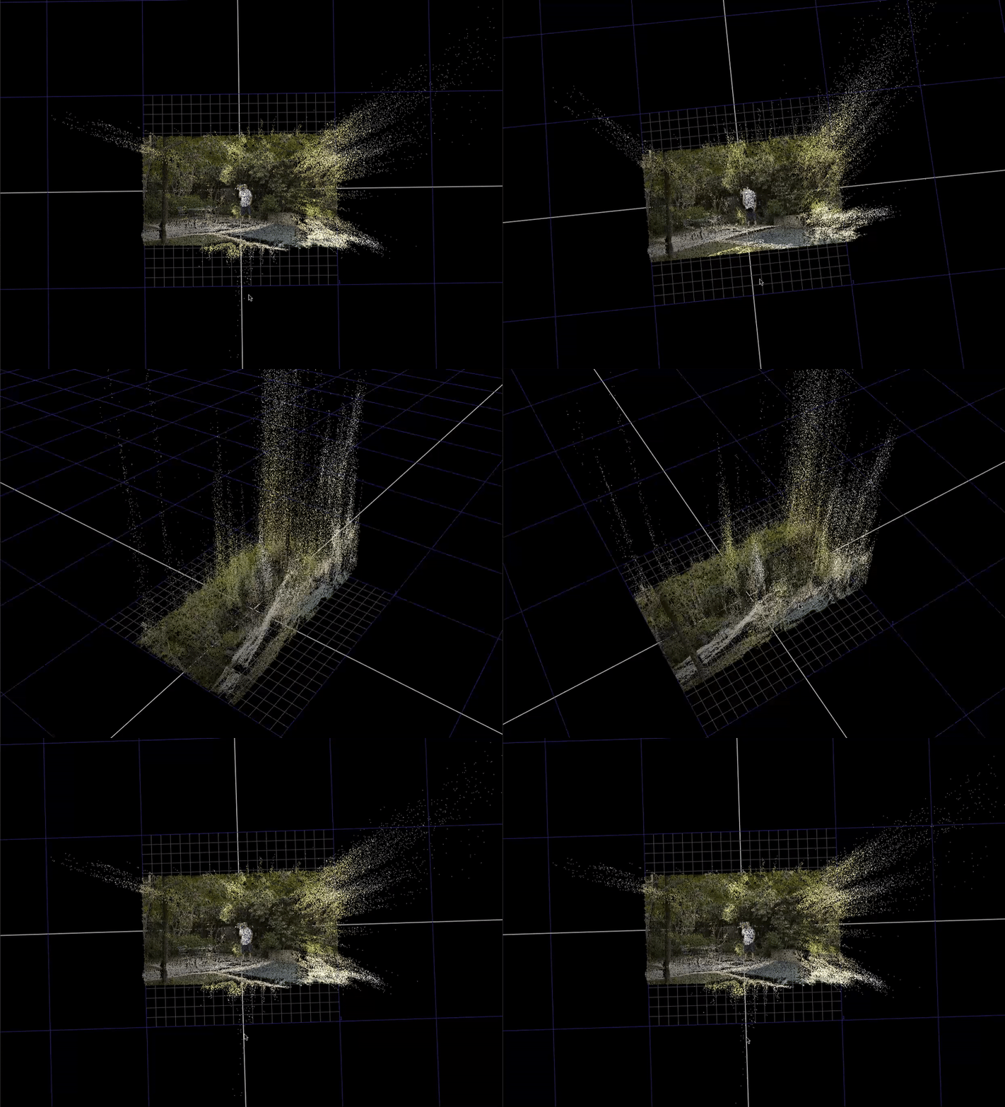
The distribution of the pixel data is interesting. The high intensity spikes are the highlights. Most of the pixel data is clumped together down there around middle grey though.
We could remap luminance intensity using a log function.
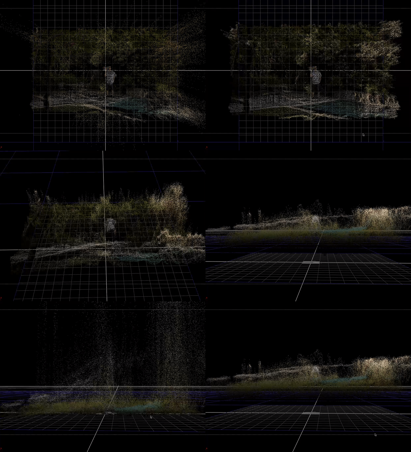
This re-distributes the intensity logarithmically, boosting midtones and shadows, and compressing those highlight spikes to be in a smaller range.
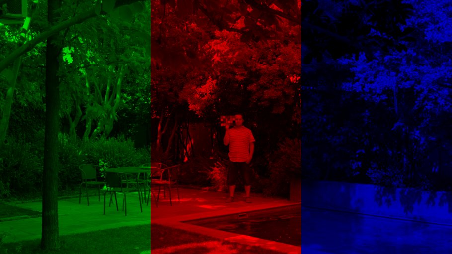
But the image data is composed of three different representations of intensity: Red Green and Blue. When the three channels are added together, it forms the illusion of color. (Even though though the spectra of the individual RGB stimulus' might be very narrow, we can't tell the difference between this and a full spectrum light source. See observer metamerism).
In 3 dimensions we could think of this like a 3-dimensional vector space. If we rotate the coordinate system so that achromatic (r=g=b) intensity is facing up: (in an XYZ coordinate system it would be an X rotation of -degrees(atan(sqrt(0.5)))), it might be a useful way to visualize the data.
Here is the same scene-linear pool guy image, but this time plotted in 3D with each R G B channel representing individual direction.
I've included the bottom half of a cube (also rotated on its axis as described above), so you can see where the edges of the 0-1 range in the vector space falls.
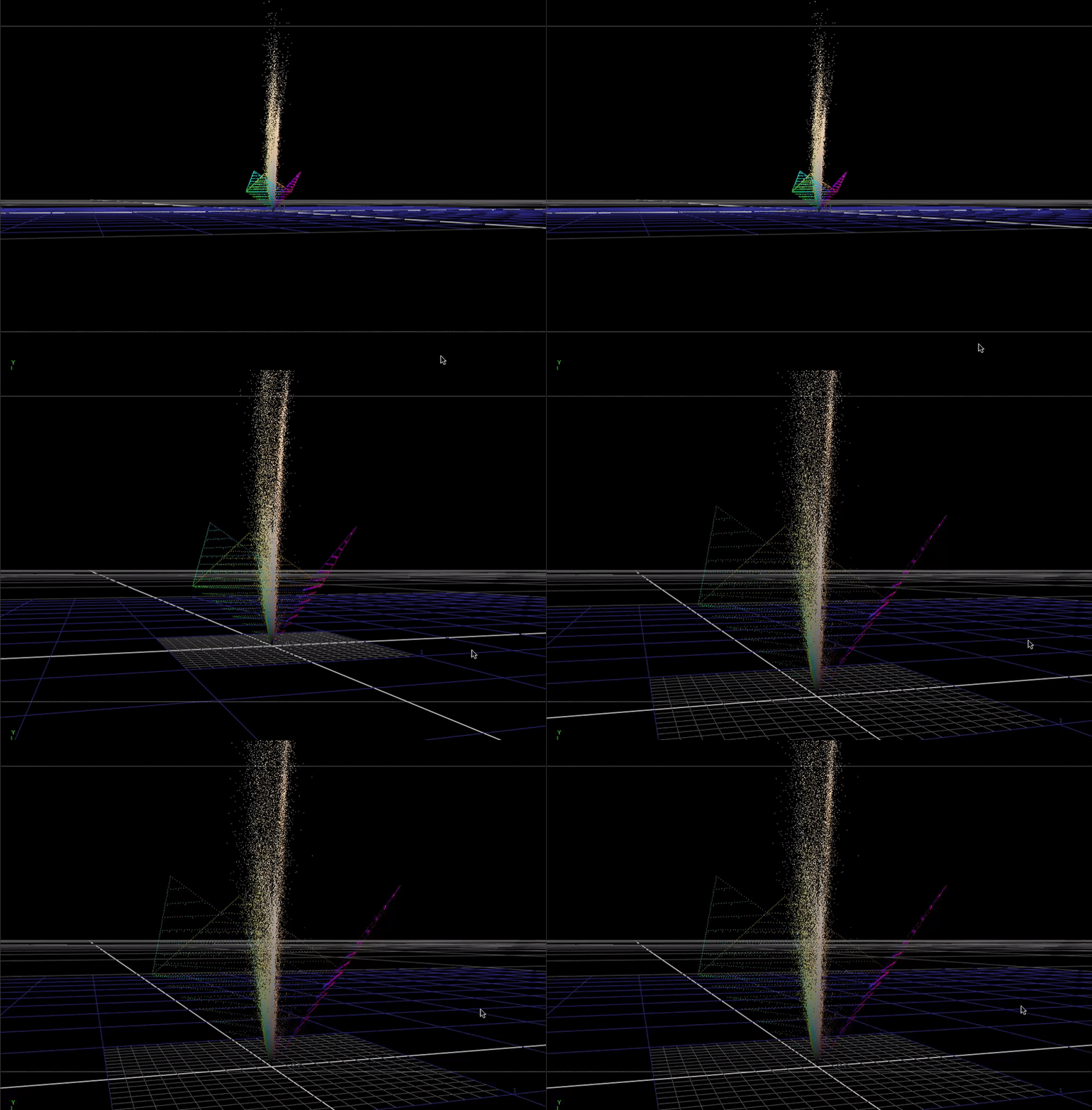
This plot is not really recognizable as an image any more, but it is useful to see how the color data in the pixels is distributed in 3D.
What if we do another plot. This time a dissolve between a gradient where r=g=b, to a fully saturated hue sweep.

If take this image and expose it up so that the max value is much higher than 1, and plot this in 3D ...
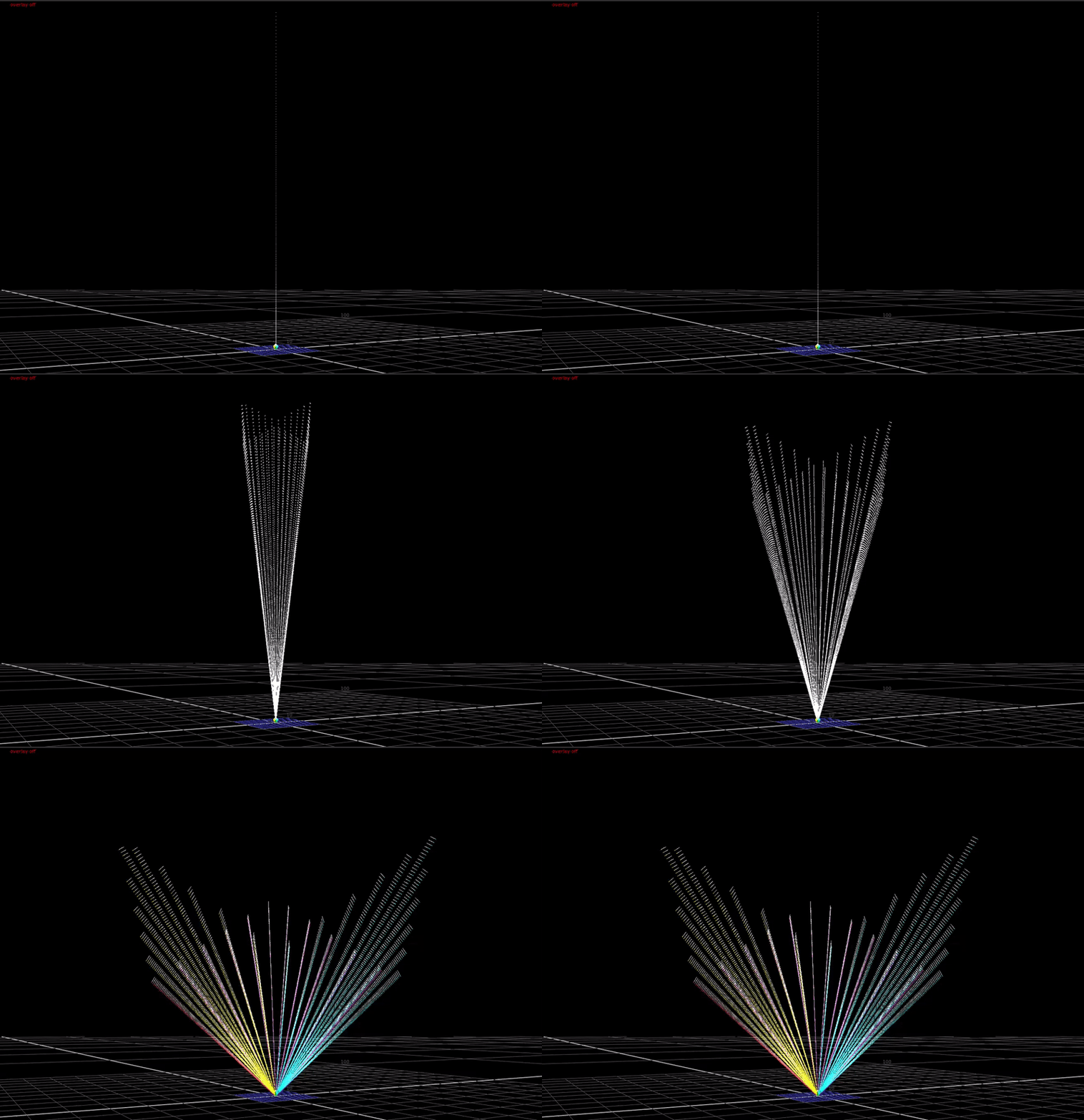
(You can just make out the 0-1 range represented by the cube down there at the bottom). This is what scene-linear data actually looks like in 3 dimensions.
But what about display-referred data? Well as mentioned before, with display-referred colorspaces, we need to put a cap on that cube, because the range of possible values is only 0-1 in each of the 3 directions.
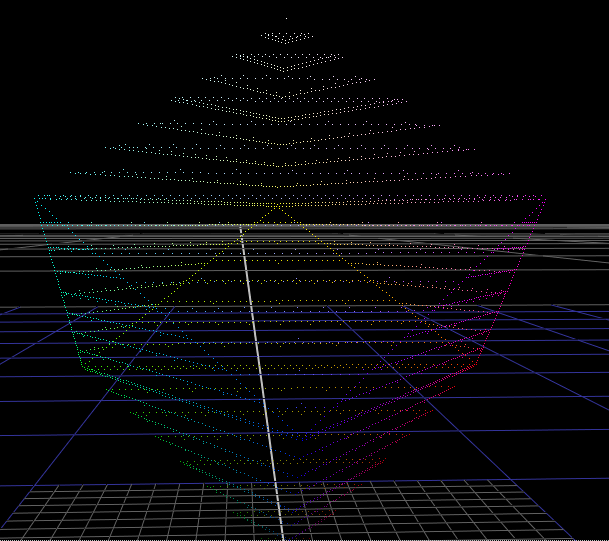
This is a bounded colorspace, as opposed to an unbounded colorspace. In this "display-referred gamut volume", values cannot exist outside of the cube.
Bullshit, you can't tell me what to do!
-- Angry Reader
Okay fine, let me prove it to you with some more animated gifs. But not in this article because it's getting too long and I'm pretty sure no one is still reading. Except for you, Angry Reader... Except for you.
Next...
