-
Notifications
You must be signed in to change notification settings - Fork 0
/
README.Rmd
180 lines (121 loc) · 6.18 KB
/
README.Rmd
1
2
3
4
5
6
7
8
9
10
11
12
13
14
15
16
17
18
19
20
21
22
23
24
25
26
27
28
29
30
31
32
33
34
35
36
37
38
39
40
41
42
43
44
45
46
47
48
49
50
51
52
53
54
55
56
57
58
59
60
61
62
63
64
65
66
67
68
69
70
71
72
73
74
75
76
77
78
79
80
81
82
83
84
85
86
87
88
89
90
91
92
93
94
95
96
97
98
99
100
101
102
103
104
105
106
107
108
109
110
111
112
113
114
115
116
117
118
119
120
121
122
123
124
125
126
127
128
129
130
131
132
133
134
135
136
137
138
139
140
141
142
143
144
145
146
147
148
149
150
151
152
153
154
155
156
157
158
159
160
161
162
163
164
165
166
167
168
169
170
171
172
173
174
175
176
177
178
179
180
---
output: github_document
bibliography: ["vignettes/packages.bib", "vignettes/PAGES.bib"]
---
<!-- README.md is generated from README.Rmd. Please edit that file -->
```{r, include = FALSE}
knitr::opts_chunk$set(
collapse = TRUE,
comment = "#>",
fig.path = "man/figures/README-"
)
```
# PAGES
<!-- badges: start -->
[](https://zenodo.org/badge/latestdoi/370009359)
<!-- badges: end -->
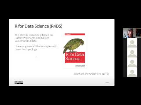
The package PAGES is the supportive material of a webinar designed for the [PAGES Early-Career Network (ECN)](http://pastglobalchanges.org/ecn/intro). The goal is to give some useful pointers to explore geological data, in particular stratigraphic occurrences, and uses RStudio and packages from the [tidyverse universe](https://www.tidyverse.org/packages/).
[](https://www.youtube.com/watch?v=r99jsChi4HU)
```{r pkgs, echo=FALSE, message=FALSE}
# following code for loading and writing the bibtex references for the used pkgs
pkgs <- c("dplyr", "tidyr", "tibble", "readr", "magrittr", "ggplot2",
"devtools", "roxygen2", "knitr", "rmarkdown", "bibtex",
"marelac", "datasauRus", "thematic")
# load
invisible(mapply(library, pkgs, character.only = TRUE))
# Get the R reference
rref <- citation()
# Create ref key
rref$key <- "rversion"
hadley <- bibentry(
key = "Wickham2015",
bibtype = "Book",
title = "R packages: organize, test, document, and share your code",
author = person("Hadley","Wickham"),
year = "2015",
publisher = " O'Reilly Media, Inc.",
url = "https://r-pkgs.org/"
)
knitr::write_bib(pkgs, "vignettes/packages.bib", prefix = "")
pkgs <- bibtex::read.bib("vignettes/packages.bib")
bibtex::write.bib(
purrr::reduce(list(rref, hadley, pkgs), append),
file = "vignettes/packages.bib"
)
# copy presentation
fs::file_copy(
fs::path("vignettes/PAGES", ext = "bib"),
fs::path("inst", "presentation", "PAGES", ext = "bib"),
overwrite = TRUE
)
fs::file_copy(
fs::path("vignettes/packages", ext = "bib"),
fs::path("inst", "presentation", "packages", ext = "bib"),
overwrite = TRUE
)
```
## R for Data Science (R4DS)
This class is modelled after Hadley Wickham's and Garrett Grolemund's R4DS. However, I have augmented the examples with cases from geology.
```{r cover, echo=FALSE, fig.cap="Book cover [@Wickham2016]", out.width="40%"}
knitr::include_graphics("man/figures/cover.png")
```
## Credits
The construction of the R [@rversion] package *PAGES* and associated documentation was aided by the packages; *devtools* [@devtools], *roxygen2* [@roxygen2], *knitr* [@knitr; @knitr2014 ; @knitr2015], *rmarkdown* [@rmarkdown; @rmarkdown2018; @rmarkdown2020], *bibtex* [@bibtex], and the superb guidance in the book: *R packages: organize, test, document, and share your code*, by @Wickham2015. In addition, this package relies on a set of external packages from the tidyverse universe, including: *dplyr* [@dplyr], *tidyr* [@tidyr], *tibble* [@tibble], *readr* [@readr], *magrittr* [@magrittr], and *readr* [@readr]. Plots are made with *ggplot2* [@ggplot2; @ggplot22016] and *thematic* [@thematic] is used for a consistent design in the presentation.
The package *marelac* [@marelac] is used for chemical data and transformations, and the package *datasauRus* [@datasauRus] is used as an example for the strength of plotting data.
## Installation
You can install the released version of PAGES from [github](https://github.io) with:
``` r
# Install PAGES from GitHub:
# install.packages("devtools")
devtools::install_github("MartinSchobben/PAGES", build_vignettes = TRUE)
```
## Usage
Load PAGES with `library`.
```{r}
library(PAGES)
```
## Data sources
The study on the Triassic--Jurassic (~201 million years before present) boundary section of Bonenburg (Germany) and Kuhjoch (Austria) by @Schobben2019 is used as the example material for this course. Lazy load datasets constitute:
-`kuhjoch` - Kuchjoch is a palynological dataset where the counts have summed for spores, pollen, aquatic and terrestrial elements.
-`bonenburg` - Bonenburg is a geochemical dataset containing: elemental analyser total organic carbon (TOC) and total nitrogen (TN), XRF element data; Aluminium (Al), Potassium (K) and sodium (Na), as well as the carbon isotope composition of TOC (del13Ctoc).
Raw datasets (`kuhjoch_raw.csv` and `bonenburg_raw.csv`) can be easily accessed with the `PAGES_example()` function and a call to the `readr` function `read_csv()`.
``` r
readr::read_csv(PAGES_example("kuhjoch_raw.csv"))
```
## Render presentation slides
To render the presentation slides:
``` r
render_slides()
```
## Exercises
Details regarding the exercise and live programming during the webinar can be found under the package vignettes (called with `vignette()`).
- RStudio projects: `vignette("project", package = "PAGES")`
- Exploratory data analysis: `vignette("explore", package = "PAGES")`
- Patterns and models: `vignette("model", package = "PAGES")`
- Load, tidy and transform data: `vignette("wrangle", package = "PAGES")`
## Tidy format
The lazy load datasets are provided in a tidy format. Look-up directory `data-raw` on the Github repository for details on the data processing.
```{r tidy}
head(bonenburg)
```
Besides wide format data the similarly named datasets with the suffix `_long` are used to generate, for example, multi-proxy stratigraphic plots for initial data exploration.
```{r strat, fig.height=4, fig.width=8, fig.cap="Bonenburg geochemical data traversing the Triassic-Jurassic boundary."}
ggplot(data = bonenburg_long) +
geom_point(mapping = aes(x = value, y = height)) +
facet_grid(cols = vars(measurement), scales = "free_x") +
theme_classic()
```
# Further reading
**Data science with R**
Hadley Wickham & Garrett Grolemund 2016 *R for Data Science*
**General statistics with R**
Peter Dalgaard 2008 *Introduction to statistics with R*
**Regression with R**
John Fox & Sanford Weisberg 2018 *An R companion to applied regression*
**Mixed effect models with R**
Alain Zuur et al. 2008 *Mixed Effects Models and Extensions in Ecology with R*
---
nocite: |
@Dalgaard2008; @Fox2018; @Zuur2008; @Wickham2016
...
# References